Dijkstra's Algorithm

Weighted Graphs

A weighted graph is a graph where each edge has a weight associated with it. The weight can represent something like: Distance, Time, Cost or Network latency

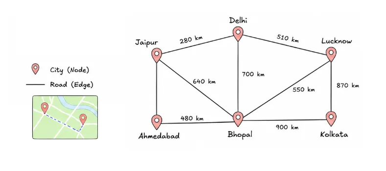
For example, in a map, cities can be represented as nodes and the distance between them as edge weights.

---

Dijkstra’s Algorithm

Breadth-First Search (BFS) finds the path with the fewest segments, but it does not consider weights that’s where Dijkstra Algo is used.

BFS asks: “Which path has the fewest steps?” Dijkstra asks: “Which path has the lowest total cost?”

How Dijkstra’s Work ?

• Dijkstra keeps track of the cheapest known cost to reach every node.
• It starts at the source node with a cost of 0. Every other node initially has an infinite cost because we do not know how to reach it yet.
• Repeatedly
  • First, find the unprocessed node with the lowest known cost.
  • Second, look at all of its neighbors and check whether going through this node gives us a cheaper path.
  • Third, mark the node as processed and continue with the next cheapest node.

We also keep track of the parent of each node. The parent allows us to reconstruct the final path once we reach the destination.

---

Example of Dijkstra: Travel from Mumbai to Chennai

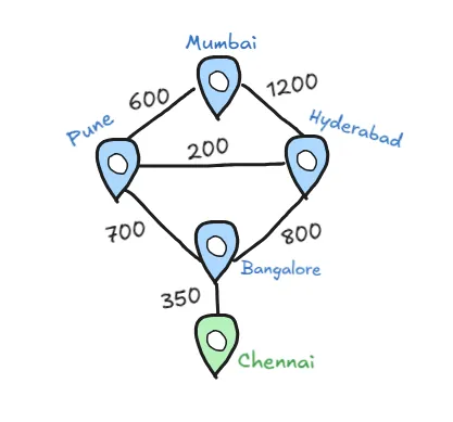
Let’s find the shortest path from Mumbai to Chennai using the graph above.

Initial State

Start at Mumbai with distance 0. Set all other unvisited cities to their direct edge cost or infinity.

City	Cost	Parent
Mumbai	0	—
Pune	600	Mumbai
Hyderabad	1200	Mumbai
Bangalore	∞	—
Chennai	∞	—

Iteration 1: Process Pune

• Pick smallest node: Pune (cost: 600 km). Mark Pune as processed.

• Update neighbors:

  • Bangalore: 600 + 700 = 1300 km (better than infinity so Update)
  • Hyderabad: 600 + 200 = 800 km (better than 1200km so Update)

City	Cost	Parent
Mumbai	0	—
Pune	600	Mumbai
Hyderabad	800	Pune
Bangalore	1300	Pune
Chennai	∞	—

Iteration 2: Process Hyderabad

• Pick smallest node: Hyderabad (cost: 800 km). Mark Hyderabad as processed.

• Update neighbors:

  • Pune: 800 + 200 = 1000km (Discarded as 1000km > 600Km)
  • Bangalore: 800 + 800 = 1600km (Discarded as 1600Km > 1300km)

(No values change in the table during this iteration)

Iteration 3: Process Bangalore

• Pick smallest node: Bangalore (cost: 1300 km). Mark Bangalore as processed.
• Update neighbors:
  • Chennai: 1300 + 350 = 1650km (better than infinity so Update)

City	Cost	Parent
Mumbai	0	—
Pune	600	Mumbai
Hyderabad	800	Pune
Bangalore	1300	Pune
Chennai	1650	Bangalore

Result: Path Reconstruction

Because Chennai is reached with no remaining cheaper paths to explore, we stop. Trace the parents backwards to reconstruct the route: Chennai → Bangalore → Pune → Mumbai

Final shortest path : Mumbai → Pune → Bangalore → Chennai ( Total dist = 1650km)

---

Dijkstra’s Implementation

function dijkstra(graph, start, destination) {
    const costs = {};
    const parents = {};
    const processed = new Set();

    // Initialize costs
    for (const node in graph) {
        costs[node] = Infinity;
        parents[node] = null;
    }

    costs[start] = 0;

    while (true) {
        // Find the cheapest unprocessed node
        let currentNode = null;
        let lowestCost = Infinity;

        for (const node in costs) {
            if (!processed.has(node) && costs[node] < lowestCost) {
                currentNode = node;
                lowestCost = costs[node];
            }
        }

        // No more reachable nodes
        if (currentNode === null) {
            break;
        }

        // Destination reached
        if (currentNode === destination) {
            break;
        }

        // Update neighbors
        for (const edge of graph[currentNode]) {
            const newCost = costs[currentNode] + edge.weight;

            if (newCost < costs[edge.node]) {
                costs[edge.node] = newCost;
                parents[edge.node] = currentNode;
            }
        }

        processed.add(currentNode);
    }

    // Destination cannot be reached
    if (costs[destination] === Infinity) {
        return null;
    }

    // Reconstruct shortest path
    const path = [];
    let currentNode = destination;

    while (currentNode !== null) {
        path.push(currentNode);
        currentNode = parents[currentNode];
    }

    path.reverse();

    return {
        path,
        cost: costs[destination]
    };
}

Time Complexity

In our implementation, we scan all nodes to find the cheapest unprocessed node.

• Time: O(V²)
• Space: O(V)

Where V is the number of nodes.

A more optimized implementation using a priority queue (min-heap) can achieve O((V + E) log V).