Dynamic Programming

Dynamic Programming (DP) is a technique for solving problems by breaking them into smaller subproblems, solving each subproblem once, and storing the result so we don’t have to calculate it again.

The core rule:

Solve smaller subproblems first, store their results, and combine them to solve the bigger problem.

Let’s see this in action using the classic 0/1 Knapsack Problem.

---

The Problem: Knapsack

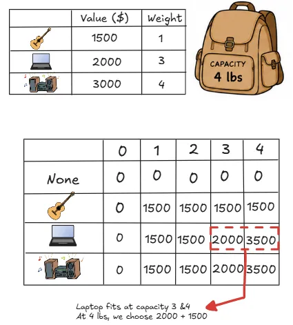
You carry a bag with a maximum capacity of 4 lbs.

A shop offers the following items:

Item	Value ($)	Weight (lbs)
Guitar	$1500	1 lb
Laptop	$2000	3 lbs
Stereo	$3000	4 lbs

Instead of testing all 2^n combinations, we build a 2D table, step by step.

• Rows represent items considered so far.
• Columns represent knapsack capacities from 0 to 4 lbs.
• Each cell answers: What is the maximum value possible with this exact capacity using only the items available so far?

At each step, we check:

1. If the item does not fit: Keep the previous best value for this capacity.
2. If the item fits: Choose the better option between:
   • Leaving it: The best value without this item.
   • Taking it: The item’s value + the best value for the remaining weight left over.

---

Step 0: Base Case (No Items)

With 0 items, the maximum possible value is always 0:

Items considered ↓ / Capacity →	0	1	2	3	4
None	0	0	0	0	0

---

Step 1: Add the Guitar (1 lb, $1500)

The Guitar weighs 1 lb and is worth $1500.

Items Considered ↓ / Capacity →	0	1	2	3	4
None	0	0	0	0	0
Guitar	0	1500	1500	1500	1500

As soon as capacity reaches at least 1 lb, we can carry the Guitar. Because no other items are available yet, the value stays $1500 across all larger capacities.

---

Step 2: Add the Laptop (3 lbs, $2000)

Items Considered ↓ / Capacity →	0	1	2	3	4
None	0	0	0	0	0
Guitar	0	1500	1500	1500	1500
Laptop	0	1500	1500	2000	3500

• At capacities 1 and 2, the Laptop (3 lbs) cannot fit, so we copy the previous best value ($1500).
• At capacity 3, the Laptop fits. We compare:
  • Leave Laptop: $1500
  • Take Laptop: $2000 + value at remaining 0 lbs ($0) = $2000
  • max(1500, 2000) = 2000$.
• At capacity 4:
  • Leave Laptop: $1500 (from previous row)
  • Take Laptop: $2000 + best value for remaining 1 lb (4 - 3 = 1) = 2000 + 1500 = 3500$
  • max(1500, 3500) = 3500.

---

Step 3: Add the Stereo (4 lbs, $3000)

Items Considered ↓ / Capacity →	0	1	2	3	4
None	0	0	0	0	0
Guitar	0	1500	1500	1500	1500
Laptop	0	1500	1500	2000	3500
Stereo	0	1500	1500	2000	3500

The Stereo only fits at capacity 4:

• Leave Stereo: $3500 (Laptop + Guitar from row above)
• Take Stereo: $3000 + best value for remaining 0 lbs (0) = 3000$
• max(3500, 3000) = 3500$.

Our optimal value sits in the bottom-right cell: $3500 (Guitar + Laptop).

---

The Core Recurrence Relation

// If the item exceeds current capacity c:
dp[i][c] = dp[i - 1][c]

// If the item fits:
dp[i][c] = Math.max(
  dp[i - 1][c],                          // Leave it
  value + dp[i - 1][c - weight]          // Take it + remaining capacity best
)

In plain English:

Best value = max(leave current item, take current item + best value for whatever space remains)

---

Javascript Implementation

function knapsack(items, capacity) {
  const n = items.length;
  // Initialize a (n + 1) x (capacity + 1) matrix with 0s
  const dp = Array.from({ length: n + 1 }, () => Array(capacity + 1).fill(0));

  for (let i = 1; i <= n; i++) {
    const { weight, value } = items[i - 1];

    for (let c = 1; c <= capacity; c++) {
      if (weight > c) {
        // Item is too heavy; carry forward previous optimal value
        dp[i][c] = dp[i - 1][c];
      } else {
        // Choose the maximum between taking or leaving the item
        dp[i][c] = Math.max(
          dp[i - 1][c],
          value + dp[i - 1][c - weight]
        );
      }
    }
  }

  return dp[n][capacity];
}

const items = [
  { weight: 1, value: 1500 }, // Guitar
  { weight: 3, value: 2000 }, // Laptop
  { weight: 4, value: 3000 }  // Stereo
];

console.log(knapsack(items, 4)); // Output: 3500